Covariate Extraction
We now continue building a spatial covariate dataset for LGCP model. Given the file `additional_city_objects.RData’ built in the previous step (see Covariate Extraction), we will compute the distances to the nearest objects and transformations based on them. The distances can be computed either using the Euclidean distance or the shortest path distance, i.e. geodesic. In this case, we will use the Euclidean distance, due to computational constraints.
1 Using the Euclidean distances
We will first start by computing the distances to the nearest objects for each accident location. Then for our Model 2, we have to additionally compute the distances to the nearest objects for each mesh location. This is a crucial step in the LGCP model, as the spatial covariates have to be available for both the accidents and the mesh locations. It is therefore crucial to select the appropriate covariates that will be available or can be computed for the whole spatial domain.
library(osmdata)
library(sf)
library(MetricGraph)
library(rSPDE)
library(INLA)
library(qs)
library(ggplot2)
library(DataExplorer)
library(here)

# Load data
df <- qread("Data/data_all_reasons_full_FRC7.qs")
graph <- qread("Data/graph_mesh_pruned_50m_7FRC.qs")
load("Data/additional_city_objects.RData")
1.1 Computing distances for each accident location
Each accident is a point with a geometry, we need to compute the distance to the nearest mosque, school, bank, fuel station, hospital. We will use the function `st_nearest_feature’ from the sf package.
######### OPTION 1 - COMPUTING THE EUCLIDEAN DISTANCES TO THE NEAREST OBJECTS #########

compute_nearest_distance <- function(points, objects) {
  distances <- st_distance(points, objects)

  # Check and print the units of the distances
  distance_units <- attr(distances, "units")
  print(paste("The units of the distances are:", distance_units))

  min_distances <- apply(distances, 1, min)
  return(min_distances)
}

accidents_sf <- st_as_sf(df, coords = c("longitude", "latitude"), crs = 4326, remove = FALSE)


##### Compute for all the accident locations #####
# Merge all of the amenities into a single data frame
objects <- rbind(mosques, education_places, finance_places, hospital_places, intersection)
amenities = c("mosque", "education", "finance", "hospital", "intersection")
for(i in amenities){
  df[[paste0("distance_to_", i)]] <- compute_nearest_distance(accidents_sf, objects %>% filter(amenity == i))
}

transform_distances <- function(distances, method = "inverse") {
  if (method == "inverse") {
    return(1 / distances)
  } else if (method == "inverse_sqrt") {
    return(1 / sqrt(distances))
  } else if (method == "log") {
    return(log1p(distances))  # log1p computes log(1 + x), handling zero distances
  } else if (method == "exp_decay") {
    decay_rate <- 0.001  # in kilometers
    return(exp(-decay_rate * distances))
  } else if (method == "exp_decay_double") {
    decay_rate <-  0.002
    return(exp(-decay_rate * distances))
  } else {
    stop("Unknown transformation method")
  }
}

# transform the distances to the nearest objects for amenities
for(i in amenities){
  df[[paste0("inv_distance_to_", i)]] <- transform_distances(df[[paste0("distance_to_", i)]], method = "inverse")
  df[[paste0("inv_sqrt_distance_to_", i)]] <- transform_distances(df[[paste0("distance_to_", i)]], method = "inverse_sqrt")
  df[[paste0("log_distance_to_", i)]] <- transform_distances(df[[paste0("distance_to_", i)]], method = "log")
  df[[paste0("exp_decay_distance_to_", i)]] <- transform_distances(df[[paste0("distance_to_", i)]], method = "exp_decay")
  df[[paste0("exp_decay_double_distance_to_", i)]] <- transform_distances(df[[paste0("distance_to_", i)]], method = "exp_decay_double")
}
Here is the code used to generate the plots:
# plot the transformed distances for the mosque and save it
png("Figures/3Covariates_all_transformations_hist_distance_to_mosque.png", height = 3*500, width = 3*700, res = 300)
par(mfrow = c(2, 3))
hist(df$inv_distance_to_mosque, main = "Inverse Distance to Nearest Mosque")
hist(df$inv_sqrt_distance_to_mosque, main = "Inverse Square Root Distance to Nearest Mosque")
hist(df$log_distance_to_mosque, main = "Log Distance to Nearest Mosque")
hist(df$exp_decay_distance_to_mosque, main = "Exponential Decay Distance to Nearest Mosque")
hist(df$exp_decay_double_distance_to_mosque, main = "Exponential Decay Double Distance to Nearest Mosque")
dev.off()

png("Figures/3Covariates_exp_decay_all_amenities.png",height = 3*500, width = 3*700,res = 300)
par(mfrow = c(2, 3))
hist(df$exp_decay_distance_to_mosque, main = "Exponential Decay Distance to Nearest Mosque")
hist(df$exp_decay_distance_to_finance, main = "Exponential Decay Distance to Nearest Bank or ATM")
hist(df$exp_decay_distance_to_hospital, main = "Exponential Decay Distance to Nearest Hospital")
hist(df$exp_decay_distance_to_intersection,  main = "Exponential Decay Distance to Nearest Intersection")
hist(df$exp_decay_distance_to_education, main = "Exponential Decay Distance to Nearest School")
dev.off()
This will be our data used in LGCP model. We will save the data and the graph with the distances to the nearest objects.
graph$add_observations(df, normalized = TRUE, tolerance =0.6, group = "YearNew",clear_obs = TRUE, duplicated_strategy = "jitter")

png("Figures/3Covariates_exp_decay_distance_to_hospital_7FRC.png",height = 3*500, width = 3*700,res = 300)
graph$plot(data = "exp_decay_distance_to_hospital", vertex_size=0, edge_width = 0.07,
           data_size = 0.5, group = c(1,2,3)) + theme_minimal() +
  ggtitle("Distance to the Nearest Hospital with Exponential Decay")+ labs(color = "")
dev.off()

png("Figures/3Covariates_exp_decay_distance_to_intersection_7FRC.png",height = 3*500, width = 3*700,res = 300)
graph$plot(data = "exp_decay_distance_to_intersection", vertex_size=0, edge_width = 0.07,
           data_size = 0.5, group = c(1,2,3)) + theme_minimal() +
  ggtitle("Distance to the Nearest Intersection with Exponential Decay")+ labs(color = "")
dev.off()

png("Figures/3Covariates_exp_decay_distance_to_education_7FRC.png",height = 3*500, width = 3*700,res = 300)
graph$plot(data = "exp_decay_distance_to_education", vertex_size=0, edge_width = 0.07,
           data_size = 0.5, group = c(1,2,3)) + theme_minimal() +
  ggtitle("Distance to the Nearest School with Exponential Decay")+ labs(color = "")
dev.off()

png("Figures/3Covariates_exp_decay_distance_to_finance_7FRC.png",height = 3*500, width = 3*700,res = 300)
graph$plot(data = "exp_decay_distance_to_finance", vertex_size=0, edge_width = 0.07,
           data_size = 0.5, group = c(1,2,3)) + theme_minimal() +
  ggtitle("Distance to the Nearest Bank or ATM with Exponential Decay")+ labs(color = "")
dev.off()

png("Figures/3Covariates_exp_decay_distance_to_mosque_7FRC.png",height = 3*500, width = 3*700,res = 300)
graph$plot(data = "exp_decay_distance_to_mosque", vertex_size=0, edge_width = 0.07,
           data_size = 0.5, group = c(1,2,3)) + theme_minimal() +
  ggtitle("Distance to the Nearest Mosque with Exponential Decay")+ labs(color = "")
dev.off()

png("Figures/3Covariates_exp_decay_double_distance_to_mosque_7FRC.png",height = 3*500, width = 3*700,res = 300)
graph$plot(data = "exp_decay_double_distance_to_mosque", vertex_size=0, edge_width = 0.07,
           data_size = 0.5, group = c(1,2,3)) + theme_minimal() +
  ggtitle("Distance to the Nearest Mosque with Exponential Decay Double")+ labs(color = "")
dev.off()
1.2 Computing distances for each mesh location
##### Compute for all the mesh locations #####
mesh_PtE = graph$get_mesh_locations() # A list or a matrix containing the mesh locations, normalized to [0,1]
mesh_loc = graph$coordinates(mesh_PtE)

mesh_locations_df <- as.data.frame(mesh_loc)
names(mesh_locations_df) <- c("x", "y")
mesh_locations_sf <- sf::st_as_sf(mesh_locations_df, coords = c("x", "y"), crs = 4326, remove = FALSE)


# Calculate distances for each type of amenity
for(i in amenities){
  mesh_locations_sf[[paste0("distance_to_", i)]] <- compute_nearest_distance(mesh_locations_sf, objects %>% filter(amenity == i))
  mesh_locations_sf[[paste0("exp_decay_distance_to_", i)]] <- transform_distances(mesh_locations_sf[[paste0("distance_to_", i)]], method = "exp_decay")
  mesh_locations_sf[[paste0("inv_distance_to_", i)]] <- transform_distances(mesh_locations_sf[[paste0("distance_to_", i)]], method = "inverse")
  mesh_locations_sf[[paste0("inv_sqrt_distance_to_", i)]] <- transform_distances(mesh_locations_sf[[paste0("distance_to_", i)]], method = "inverse_sqrt")
  mesh_locations_sf[[paste0("log_distance_to_", i)]] <- transform_distances(mesh_locations_sf[[paste0("distance_to_", i)]], method = "log")
  mesh_locations_sf[[paste0("exp_decay_double_distance_to_", i)]] <- transform_distances(mesh_locations_sf[[paste0("distance_to_", i)]], method = "exp_decay_double")
}

mesh_locations_sf$.edge_number = mesh_PtE[,1]
mesh_locations_sf$.distance_on_edge = mesh_PtE[,2]

# Save the updated mesh locations with distances
qsave(mesh_locations_sf, "Data/mesh_locations_pruned_50m_with_distances_7FRC.qs")
Here is the code used to generate the plots:
png("Figures/3Covariates_exp_decay_double_distance_to_mosque_mesh_7FRC.png",height = 3*500, width = 3*700,res = 300)
ggplot(mesh_locations_sf) +
  geom_sf(aes(color = exp_decay_double_distance_to_mosque), size = 0.005) +
  scale_color_viridis_c() +
  theme_minimal() +
  labs(title = "Distance to the Nearest Mosque with Exponential Decay Double", color = "")
dev.off()

png("Figures/3Covariates_exp_decay_double_distance_to_hospital_mesh_7FRC.png",height = 3*500, width = 3*700,res = 300)
ggplot(mesh_locations_sf) +
  geom_sf(aes(color = exp_decay_double_distance_to_hospital), size = 0.005) +
  scale_color_viridis_c() +
  theme_minimal() +
  labs(title = "Distance to the Nearest Hospital with Exponential Decay Double", color = "")
dev.off()

png("Figures/3Covariates_exp_decay_double_distance_to_intersection_mesh_7FRC.png",height = 3*500, width = 3*700,res = 300)
ggplot(mesh_locations_sf) +
  geom_sf(aes(color = exp_decay_double_distance_to_intersection), size = 0.005) +
  scale_color_viridis_c() +
  theme_minimal() +
  labs(title = "Distance to the Nearest Intersection with Exponential Decay Double", color = "")
dev.off()

png("Figures/3Covariates_exp_decay_double_distance_to_education_mesh_7FRC.png",height = 3*500, width = 3*700,res = 300)
ggplot(mesh_locations_sf) +
  geom_sf(aes(color = exp_decay_double_distance_to_education), size = 0.005) +
  scale_color_viridis_c() +
  theme_minimal() +
  labs(title = "Distance to the Nearest School with Exponential Decay Double", color = "")
dev.off()

png("Figures/3Covariates_exp_decay_distance_to_mosque_mesh_7FRC.png",height = 3*500, width = 3*700,res = 300)
ggplot(mesh_locations_sf) +
  geom_sf(aes(color = exp_decay_distance_to_mosque), size = 0.005) +
  scale_color_viridis_c() +
  theme_minimal() +
  labs(title = "Distance to the Nearest Mosque with Exponential Decay", color = "")
dev.off()

png("Figures/3Covariates_exp_decay_distance_to_education_mesh_7FRC.png",height = 3*500, width = 3*700,res = 300)
ggplot(mesh_locations_sf)+
  geom_sf(aes(color = exp_decay_distance_to_education), size = 0.05) +
  scale_color_viridis_c() +
  theme_minimal() +
  labs(title = "Distance to the Nearest Bank or ATM with Exponential Decay", color = "")
dev.off()

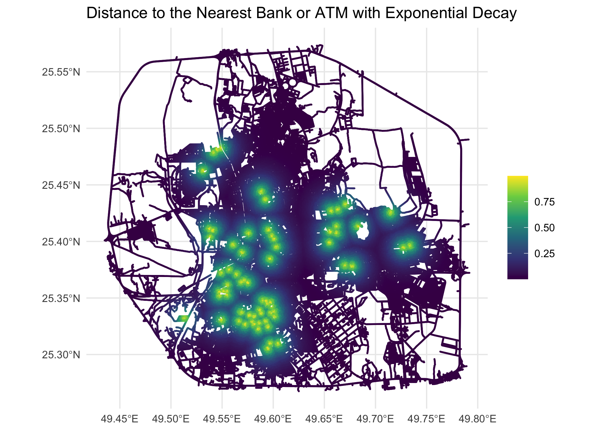
png("Figures/3Covariates_exp_decay_distance_to_finance_mesh_7FRC.png",height = 3*500, width = 3*700,res = 300)
ggplot(mesh_locations_sf)+
  geom_sf(aes(color = exp_decay_distance_to_finance), size = 0.05) +
  scale_color_viridis_c() +
  theme_minimal() +
  labs(title = "Distance to the Nearest Bank or ATM with Exponential Decay", color = "")
dev.off()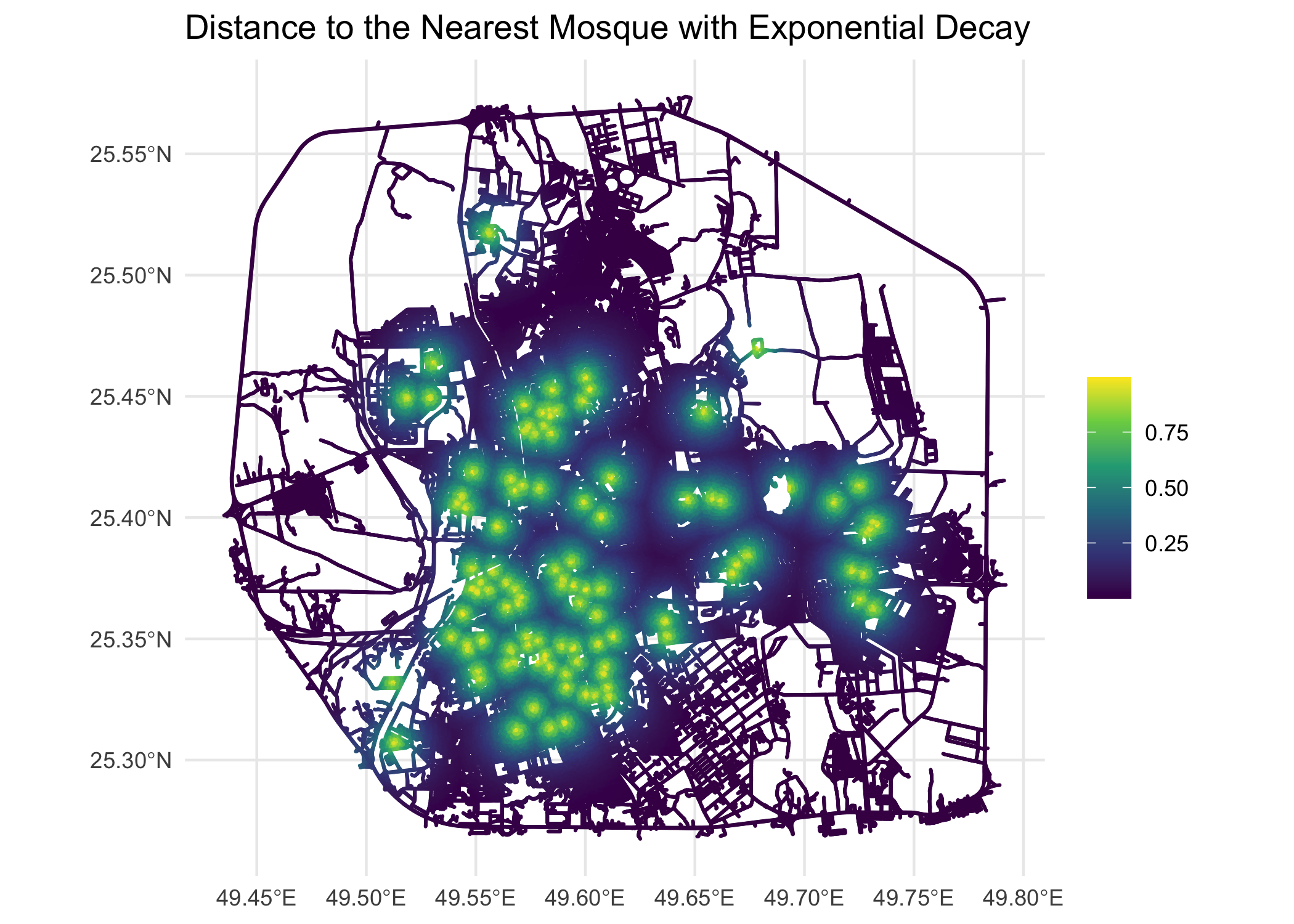
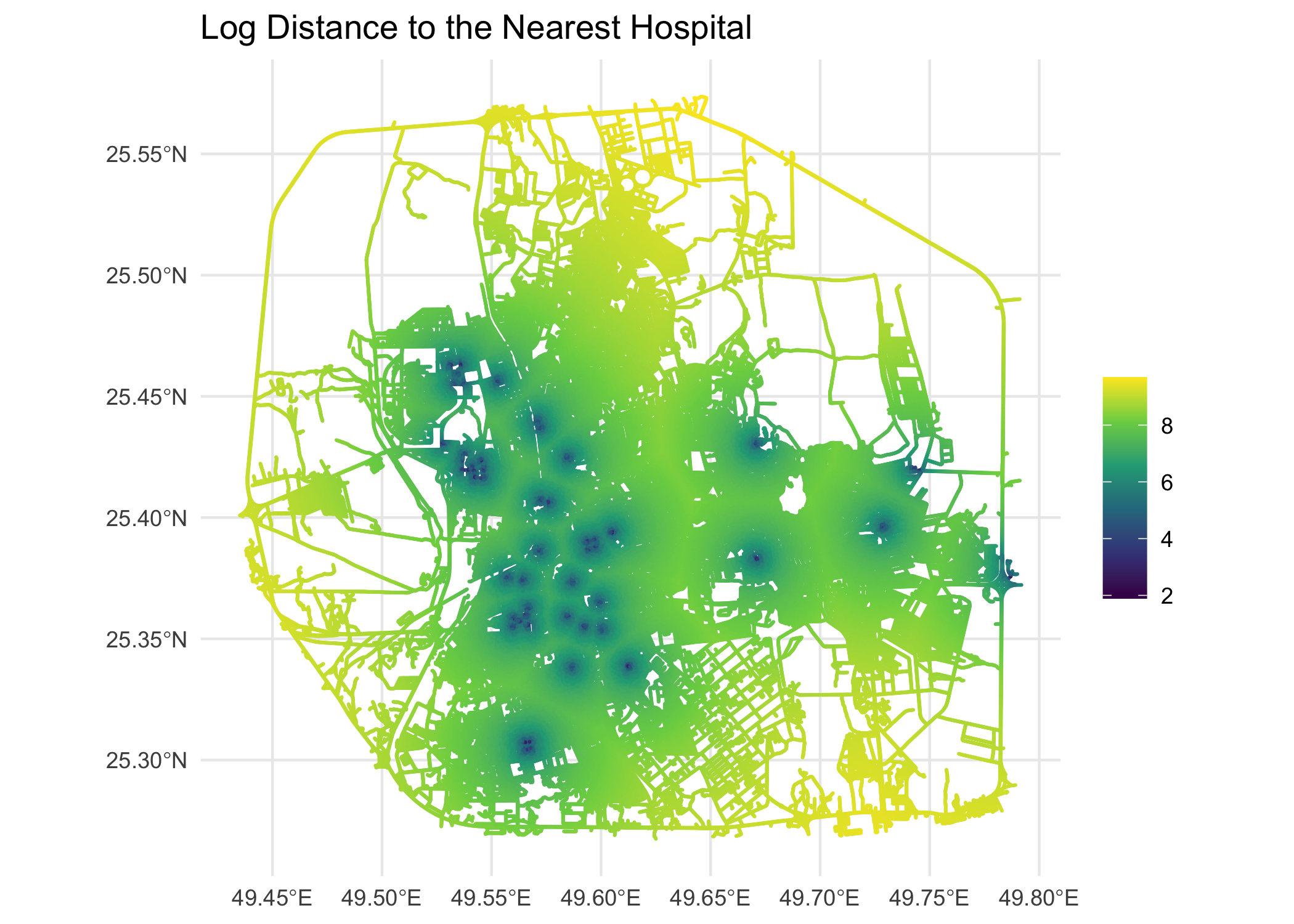
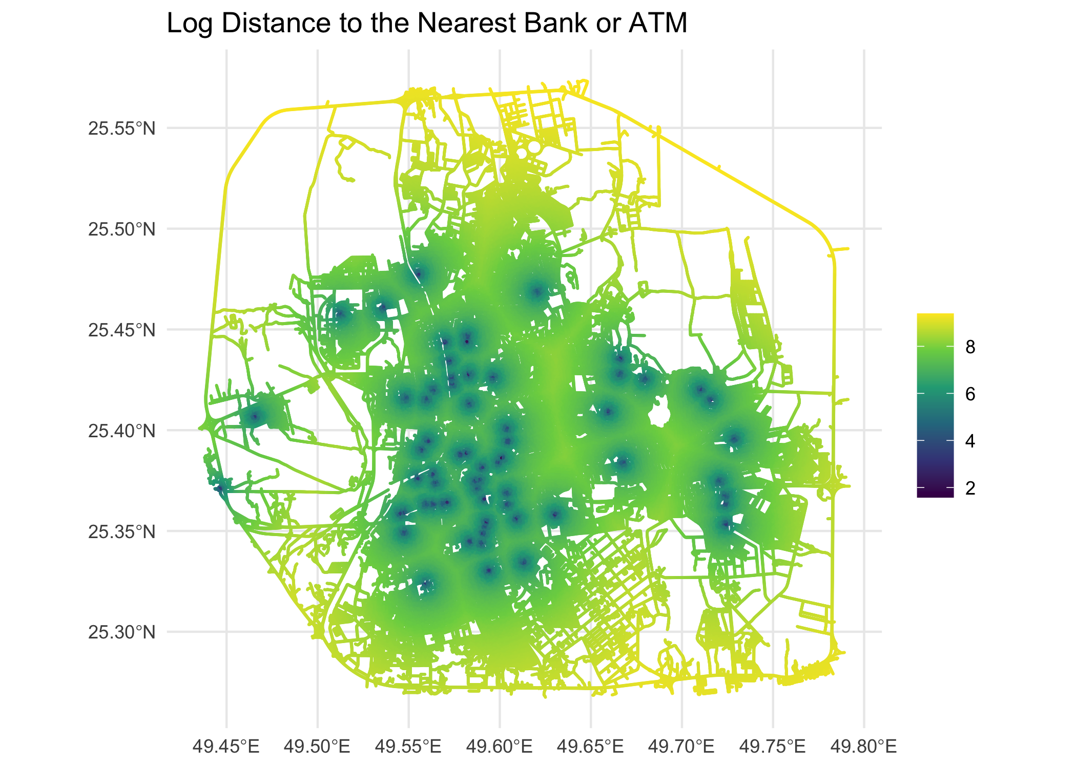
After exploring several transformations, we chose the log transformation for the final model (Model 2), as it accounts for the diminishing influence of more distant features while maintaining interpretable coefficients. The log-transformed distances to hospitals and financial institutions at mesh locations are shown below.
# plot log distances
# Log distance to mosque
png("Figures/3Covariates_log_distance_to_mosque_mesh_7FRC.png", height = 3*500, width = 3*700, res = 300)
ggplot(mesh_locations_sf) +
  geom_sf(aes(color = log_distance_to_mosque), size = 0.005) +
  scale_color_viridis_c() +
  theme_minimal() +
  labs(title = "Log Distance to the Nearest Mosque", color = "")
dev.off()

# Log distance to hospital
png("Figures/3Covariates_log_distance_to_hospital_mesh_7FRC.png", height = 3*500, width = 3*700, res = 300)
ggplot(mesh_locations_sf) +
  geom_sf(aes(color = log_distance_to_hospital), size = 0.005) +
  scale_color_viridis_c() +
  theme_minimal() +
  labs(title = "Log Distance to the Nearest Hospital", color = "")
dev.off()

# Log distance to intersection
png("Figures/3Covariates_log_distance_to_intersection_mesh_7FRC.png", height = 3*500, width = 3*700, res = 300)
ggplot(mesh_locations_sf) +
  geom_sf(aes(color = log_distance_to_intersection), size = 0.005) +
  scale_color_viridis_c() +
  theme_minimal() +
  labs(title = "Log Distance to the Nearest Intersection", color = "")
dev.off()

# Log distance to finance
png("Figures/3Covariates_log_distance_to_finance_mesh_7FRC.png", height = 3*500, width = 3*700, res = 300)
ggplot(mesh_locations_sf) +
  geom_sf(aes(color = log_distance_to_finance), size = 0.005) +
  scale_color_viridis_c() +
  theme_minimal() +
  labs(title = "Log Distance to the Nearest Bank or ATM", color = "")
dev.off()

# education
png("Figures/3Covariates_log_distance_to_education_mesh_7FRC.png", height = 3*500, width = 3*700, res = 300)
ggplot(mesh_locations_sf) +
  geom_sf(aes(color = log_distance_to_education), size = 0.002) +
  scale_color_viridis_c() +
  theme_minimal() +
  labs(title = "Log Distance to the Nearest School", color = "")
dev.off()
# education
png("Figures/3Covariates_log_distance_to_education_mesh_7FRC.png",
    height = 3*500, width = 3*700, res = 300)
ggplot(mesh_locations_sf) +
  geom_sf(aes(color = log_distance_to_education), size = 0.1) +
  scale_color_viridis_c(option = "viridis") +
  theme_minimal() +
  theme(
    plot.title = element_text(hjust = 0.5, size = 14),
    legend.position = "right",
    axis.text = element_text(size = 9),
    axis.title = element_text(size = 11)
  ) +
  labs(
    title = "Log-Transformed Distance to Nearest Educational Institution",
    color = "Log Distance",
    x = "Longitude",
    y = "Latitude"
  )
dev.off()